
Industry generally works with two kinds of equipment: static equipment (heat exchangers, cyclone separators and so on) and rotating equipment (pumps, fans, mixers and so on). Fans, and centrifugal fans in particular (often called squirrel-cage fans), are among the most common rotating machines in industry. Their simple design makes them easier to manufacture than other fan types, saving both time and cost. They are therefore widely used for ventilation (HVAC), furnace air supply, pneumatic conveying and more.
When choosing a fan for HVAC applications, most engineers pick a centrifugal fan for its good energy efficiency (static efficiency up to 84%), durability even in corrosive environments, ease of maintenance and its wide range of working flow and pressure.
How can centrifugal fan performance be predicted?
One of the strengths of a centrifugal fan is its aerodynamic behavior — an important factor to consider during design if the fan's efficiency is to be maximized. Various design-support methods can be used for that; CFD simulation is an effective one.
CFD can predict fan performance accurately at the early design stage, analyze different CAD models, cut the number of prototypes that need testing, and optimize the design for maximum efficiency. The results give accurate figures for flow rate, static head, total head, static efficiency, total efficiency, peak total efficiency, and the forces and moments acting on the fan.
To illustrate clearly what CFD can do in assessing centrifugal fan performance, this article works through a specific analysis of an industrial centrifugal fan used in a biomass-fired boiler system.
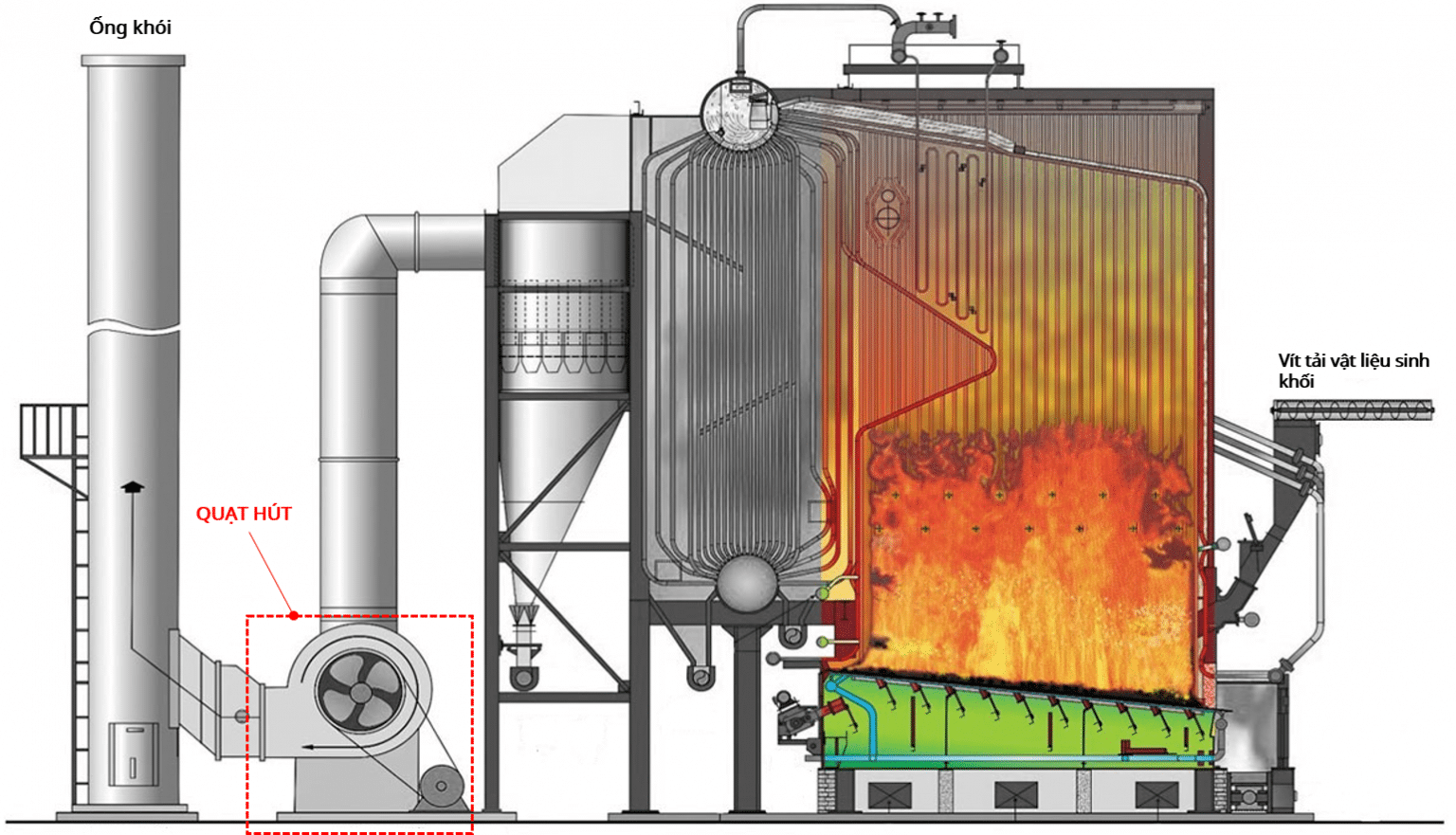
Where the induced-draft fan sits in a steam boiler system [source]
The fan performance case
A boiler turns water into steam using the heat released by burning fuel — coal, oil, natural gas or biomass. A boiler system uses several fans to maintain and circulate air and to remove the flue gas. The fan analyzed here is an induced-draft fan at the outlet of the boiler system, usually between the dust filter and the stack. It creates suction (negative pressure) to expel the gas after combustion. The most common fan types used for this duty are centrifugal fans with radial blades and with backward-inclined blades. The performance of this centrifugal fan is predicted at its steady operating point in the system (constant flow rate and constant rotational speed).
Fan geometry
- A spiral volute casing, largest dimension ~ 1 m
- Impeller diameter = 0.5 m
- Straight inclined blades, number of blades = 12
- Inlet diameter = 0.32 m, outlet size = 0.45×0.35 m
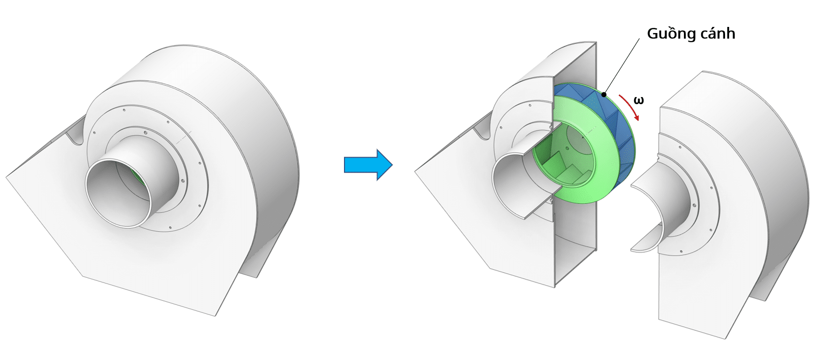
The original fan geometry (left) and a half-section of the casing showing the impeller (right)
Operating conditions
- The gas conveyed is air at 30oC (density = 1.1644 kg/m3)
- Required extraction flow = 3400 m3/h (~ 1 kg/s)
- Impeller speed = 1500 rpm
CFD simulation of the centrifugal fan
The basic steps for this simulation:
1. Geometry simplification:
The original fan geometry has to be reduced to the fluid volume (here, air at 30oC) — the computational domain. The figure below shows the whole casing simplified into a single surface, which must be the inner surface in direct contact with the fluid. The impeller is left as it is, because every one of its surfaces touches the fluid. Additional surfaces are added to carry the boundary conditions: the blue surface is the inlet and the red one the outlet.
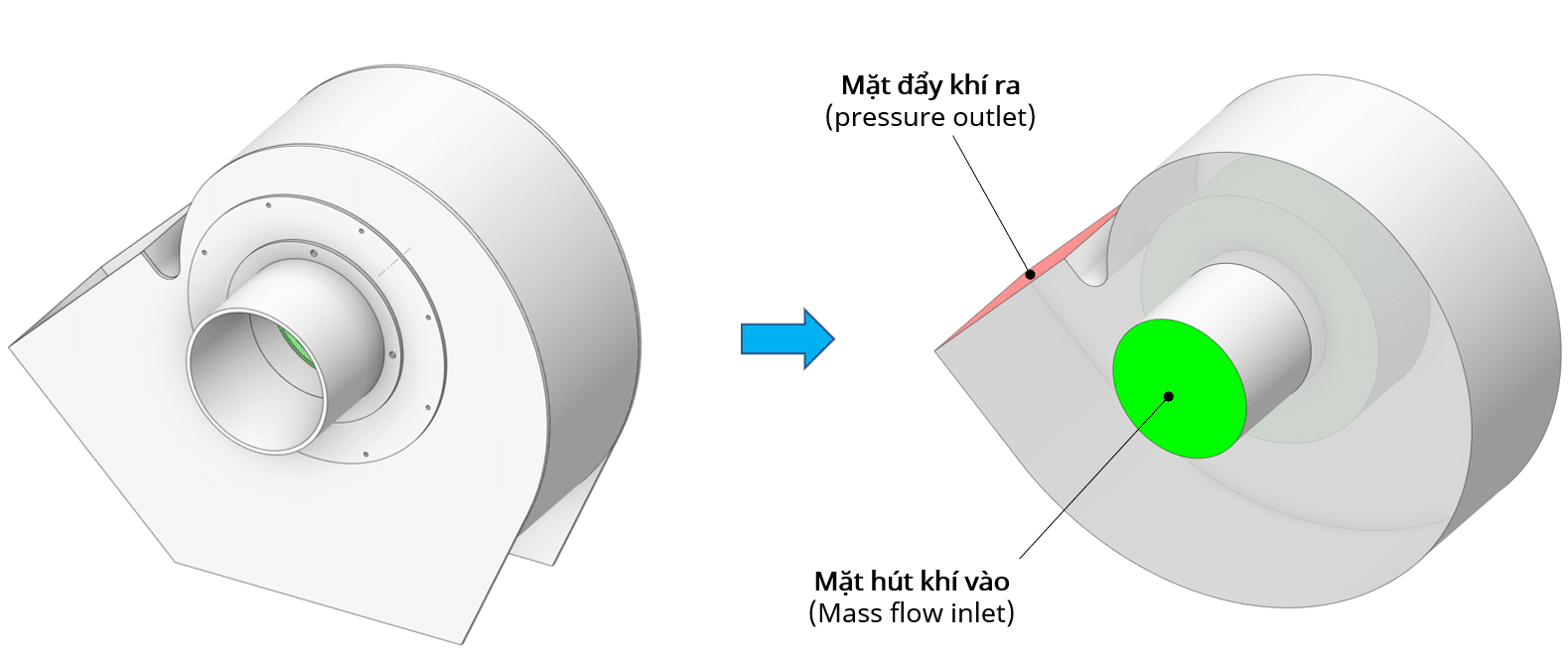
Simplifying the fan geometry
2. Mesh generation:
Meshing — discretizing the computational domain — divides it into finite volume elements. The mesh type used here is polyhedral. The total cell count is 2 million; the smallest cell is 2 mm (mostly in the impeller) and the largest 20 mm.
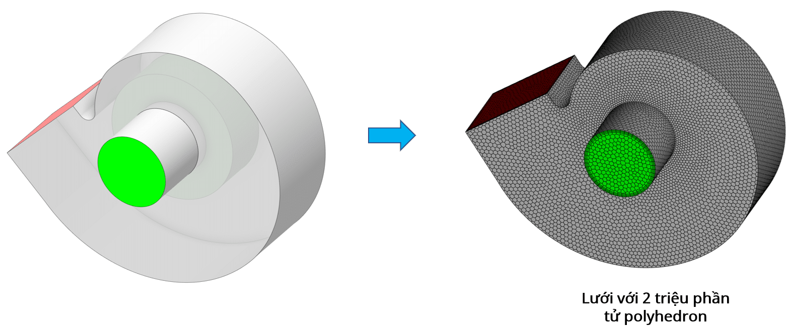
Meshing the computational domain
3. Model setup:
Assuming no heat transfer and no mass transfer, this is a CFD problem for single-phase flow (air) inside the fan. Given the turbulent nature of the flow, a turbulence model is used: Realizable k-epsilon, chosen for its fairly high accuracy and low computing cost. To model the rotating impeller, the MRF (Moving Reference Frame) model is used. Applying MRF requires a separate rotating region around the impeller; instead of setting the impeller mesh itself “in motion”*, its frame of reference is set to rotate relative to the absolute frame of the casing. MRF suits a fan simulated at a steady operating point, as here.
4. Boundary conditions setup:
Assuming incompressible flow, the inlet is given a fixed mass flow inlet boundary condition of 1 kg/s with gauge pressure = 0 to secure the required flow through the fan. The outlet is set to a gauge pressure of 82 Pa (the pressure loss of the outlet duct). The rotating region and the impeller surfaces are set to 1500 rpm with the MRF method.
5. Solver setup and run:
(1) Choose the solution method (Coupled solver, second-order accuracy).
(2) Initialize the field (initial variable value x = x0).
(3) Choose the number of iterations and start solving.
(4) Stop at the iteration where the residual is acceptable — usually described as converged. That value rests largely on experience and depends on the type of problem, the model and so on.
6. Extracting the results:
Some of the important results when analyzing centrifugal fan performance — head pressure, velocity distribution in the impeller and aerodynamic efficiency — are presented here.
- Head pressure
With a centrifugal fan working in extraction, we expect the total pressure (static + dynamic) at the inlet to be lower than at the outlet. The figure below shows the total pressure distribution over the casing and at the inlet and outlet. The head (pt) is computed from the average difference between the outlet (pt2) and the inlet (pt1):
pt = pt2 − pt1 = 82 − (−770) = 852 [Pa]
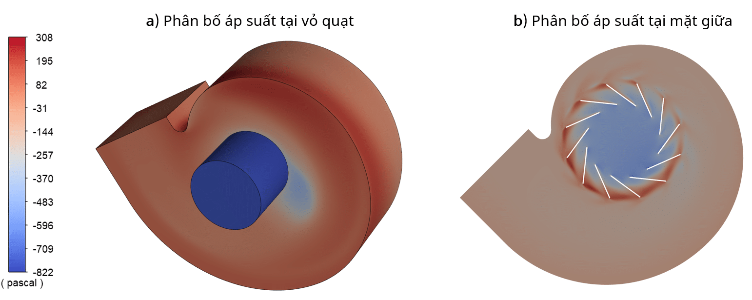
Total pressure distribution in the fan
- Velocity distribution in the impeller
The velocity distribution supports a preliminary judgement of how aerodynamically good the blade design is. Flow separation behind each blade (see the figure below) is the indicator to look at. In fan design and optimization, the less separation there is, the higher the fan efficiency.
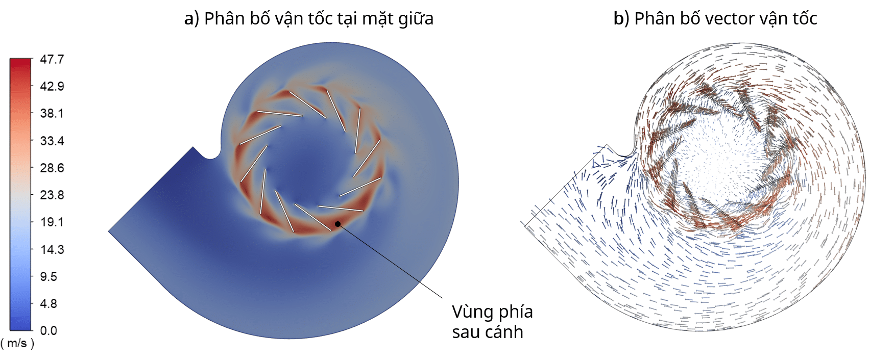
Velocity distribution in the impeller
- Aerodynamic efficiency
The aerodynamic efficiency of a fan excludes other losses such as bearing friction, the motor and the drive. It is the ratio between the aerodynamic power and the impeller torque power.
+ The aerodynamic power (Pu) is computed from the pressure rise (pt) — here the suction head — and the volumetric flow through the fan (Qv):
Pu = ptQv = 852 [Pa] × 1/1.1644 [m3/s] = 732 [W]
+ The torque power (Pr) is the product of the impeller torque (taken directly from the CFD results) and the angular velocity:
Pr = Mcω = 10.32 [Nm] × 1500 × 2π/60 [rad/s] = 1621 [W]
The aerodynamic efficiency of the fan (η) is therefore:
ηfan = Pu/Pr = 732/1621 = 45%
Running at 3400 m3/h of air (at 30oC) and 1500 rpm, the fan as designed reaches an aerodynamic efficiency of only 45%.
Conclusion
Using CFD, the performance of a centrifugal fan has been analyzed at a preliminary level through its operating characteristics. The results are useful for assessing and then optimizing the fan design (blades, impeller, casing and so on) so its behavior — suction and discharge pressure, flow rate, energy efficiency — matches what the process system requires. This analysis covers one specific operating point. Assessing the fan across a wide operating range requires its characteristics at different conditions, expressed as the “fan performance curve”. How that curve is built using CFD will be covered in a later article.
*The moving mesh method, also called “sliding mesh”, can also be used for problems with a rotating region, but it needs considerably more computing time to converge. For problems where the flow has to be analyzed as it changes in time (transient), sliding mesh is the method to use.